Machine Learning: The Mathematics of Support Vector Machines - Part 1

Introduction

The purpose of this post is to discuss the mathematics of support vector machines (SVMs) in detail, in the case of linear separability.

Background

SVMs are a tool for classification. The idea is that we want to find two lines (linear equations) so that a given set of points are linearly separable according to a binary classifier, coded as \(\pm 1\), assuming such lines exist. These lines are given by the black lines given below.

library(ggplot2)
set.seed(45)

plus_1 <- data.frame(x = runif(100, min = -3, max = 3))
plus_1$y <- plus_1$x + runif(100, min = 1.1, max = 2)

minus_1 <- data.frame(x = runif(100, min = -3, max = 3))
minus_1$y <- minus_1$x + runif(100, min = -2, max = -1.1)

ggplot() +
  geom_point(data = plus_1,
             aes(x = x, y = y),
             alpha = 0.1) +
  geom_point(data = minus_1,
             aes(x = x, y = y),
             alpha = 0.1) +
  geom_text(aes(x = 2, y = 3.5, label = "y = 1"),
            color = "black") + 
  stat_function(fun = function(x){ x + 1.142233 }, 
                color = "black",
                linetype = "dashed") +
  geom_text(aes(x = 2, y = 2.5, label = "y = 0"),
            color = "red") + 
  stat_function(fun = function(x){ x + 0.0149345 }, 
                color = "red") +
  geom_text(aes(x = 2, y = 1.5, label = "y = -1"),
            color = "black") + 
  stat_function(fun = function(x){ x - 1.112364 }, 
                color = "black",
            linetype = "dashed") +
  theme_void() + 
  scale_x_continuous(limits = c(-3, 3)) +
  scale_y_continuous(limits = c(-5, 5))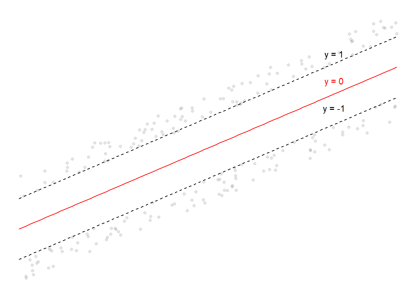 

Points at or above the \(y = 1\) line are classified as \(+1\), and points at or below the \(y = -1\) line are classified as \(-1\). The line labeled “\(y = 0\)” is known as the decision boundary. The \(y = 1\) and \(y = -1\) lines are the lines touching the points which are closest to the decision boundary.

Assuming the lines above all have common parameter vector \(\boldsymbol\beta \in \mathbb{R}^p \setminus \{\mathbf{0}\}\) (which we assume only includes the slope-related terms) and intercept term \(\beta_0 \in \mathbb{R}\), we seek the decision boundary following the form of a linear equation: \(\boldsymbol\beta^{T}\mathbf{x} + \beta_0\). At the decision boundary, we assume the classifier is \(0\), hence we assume \(\boldsymbol\beta^{T}\mathbf{x} + \beta_0 = 0\) at the decision boundary.

Let \((\mathbf{x}_1, y_1), \dots, (\mathbf{x}_N, y_N)\) denote the training data in \(\mathbb{R}^{p} \times \{-1, 1\}\), with each \(y_i \in \{-1, +1\}\) for each \(i = 1, \dots, N\). Let \(\omega_{+1}\), \(\omega_{-1}\) denote the subsets of \(\mathbb{R}^p\) for which the corresponding classifiers are \(+1\) and \(-1\) respectively. Then we assume that \[\begin{align*} &\boldsymbol\beta^{T}\mathbf{x}_i + \beta_0 \geq 1\text{, }\quad \mathbf{x}_i \in \omega_{+1} \\ &\boldsymbol\beta^{T}\mathbf{x}_i + \beta_0 \leq -1\text{, }\quad \mathbf{x}_i \in \omega_{-1} \end{align*}\] Since \(y_i \in \{-1, +1\}\), the above two conditions are equivalent to \[\begin{equation*} y_i(\boldsymbol\beta^{T}\mathbf{x}_i + \beta_0) \geq 1\text{, } \quad\mathbf{x}_i \in \mathbb{R}^{p}\text{.} \end{equation*}\] However, it is worth noting there are infinitely many possible decision boundaries that satisfy these conditions. We have to choose some sort of criteria for optimality.

An Intermediate Result

Consider the decision boundary \(\boldsymbol\beta^{T}\mathbf{x} + \beta_0 = 0\) and a point \(\mathbf{z} = \begin{bmatrix} z_1 & z_2 & \cdots & z_{p} \end{bmatrix}^{T}\in \mathbb{R}^{p}\). We aim to calculate the perpendicular distance from \(\mathbf{z}\) to \(\mathbf{x}\), given the constraint \(\boldsymbol\beta^{T}\mathbf{x} + \beta_0 = 0\). Consider minimizing the squared Euclidean distance from \(\mathbf{x}\) to \(\mathbf{z}\) subject to \(\mu(\mathbf{x}) = \boldsymbol\beta^{T}\mathbf{x} + \beta_0 = 0\), by the method of Lagrange multipliers. We work with the function \[\begin{align*} L(\mathbf{x}, \lambda) = \sum_{i=1}^{p}(x_i - z_i)^2 + \lambda\left(\beta_1x_1 + \cdots + \beta_px_p + \beta_0\right)\text{.} \end{align*}\] Then \[\begin{equation*} \dfrac{\partial L}{\partial x_i} = 2(x_i - z_i) + \lambda\beta_i = 0 \implies (x_i -z_i)^2 = \dfrac{\lambda^2\beta_i^2}{4}\text{.} \end{equation*}\] Because \(\beta_1x_1 + \cdots + \beta_px_p + \beta_0 = 0\), we have that \[\begin{equation*} \sum_{i=1}^{p}\beta_ix_i + \beta_0 = \sum_{i=1}^{p}\left(z_i\beta_i-\dfrac{\lambda\beta_i^2}{2}\right) + \beta_0 = \sum_{i=1}^{p}z_i\beta_i-\dfrac{\lambda}{2}\sum_{j=1}^{p}\beta_j^2 + \beta_0 = 0\text{.} \end{equation*}\] This implies that \[\begin{equation*} \lambda = \dfrac{2}{\sum_{j=1}^{p}\beta_j^2}\left(\beta_0 + \sum_{i=1}^{p}z_i\beta_i\right) = \dfrac{2}{\|\boldsymbol\beta\|^2_2}\mu(\mathbf{z}) \implies \dfrac{\lambda^2\beta_i^2}{4} = \dfrac{[\mu(\mathbf{z})]^2\beta_i^2}{\|\boldsymbol\beta\|_2^4}\text{.} \end{equation*}\] The squared Euclidean distance is then given by \[\begin{equation*} \sum_{i=1}^{p}(x_i - z_i)^2 = \dfrac{[\mu(\mathbf{z})]^2}{\|\boldsymbol\beta\|_2^4}\sum_{i=1}^{p}\beta_i^2 = \dfrac{[\mu(\mathbf{z})]^2\|\boldsymbol\beta\|_2^2}{\|\boldsymbol\beta\|_2^4} = \dfrac{[\mu(\mathbf{z})]^2}{\|\boldsymbol\beta\|_2^2} \end{equation*}\] hence the Euclidean distance from \(\mathbf{x}\) to \(\mathbf{z}\) is given by \[\begin{equation*} \sqrt{\sum_{i=1}^{p}(x_i - z_i)^2} = \dfrac{|\mu(\mathbf{z})|}{\|\boldsymbol\beta\|_2}\text{.} \end{equation*}\]

Optimality in SVMs

Now suppose \(\mathbf{x}_{+1}\) and \(\mathbf{x}_{-1}\) are the closest points to the decision boundary with classifications \(+1\) and \(-1\) respectively. We obtain that \[\begin{align*} &\boldsymbol\beta^{T}\mathbf{x}_{+1} + \beta_0 = 1 \\ &\boldsymbol\beta^{T}\mathbf{x}_{-1} + \beta_0 = -1\text{.} \end{align*}\] Hence, the perpendicular distances of these two points to any point \(\mathbf{x}\) on the decision boundary is given by \[\begin{align*} &\dfrac{|\mu(\mathbf{x}_{+1})|}{\|\boldsymbol\beta\|_2} = \dfrac{|\boldsymbol\beta^{T}\mathbf{x}_{+1} + \beta_0|}{\|\boldsymbol\beta\|_2} = \dfrac{1}{\|\boldsymbol\beta\|_2} \\ &\dfrac{|\mu(\mathbf{x}_{-1})|}{\|\boldsymbol\beta\|_2} = \dfrac{|\boldsymbol\beta^{T}\mathbf{x}_{-1} + \beta_0|}{\|\boldsymbol\beta\|_2} = \dfrac{1}{\|\boldsymbol\beta\|_2} \text{.} \end{align*}\] The sum of these two distances, given by \(M = \dfrac{2}{\|\boldsymbol\beta\|_2}\), is called the margin. Geometrically, one can think of the margin as the total perpendicular distances from the decision boundary to the closest points (\(\mathbf{x}_{+1}\), \(\mathbf{x}_{-1}\)) of each of the states of the binary classifier. These points are known as the support vectors.

The optimization problem with regard to SVMs is \[\begin{align*} &\max \dfrac{2}{\|\boldsymbol\beta\|_2}\\ &\text{subject to }y_i(\boldsymbol\beta^{T}\mathbf{x}_i + \beta_0) \geq 1\text{, } i = 1, \dots, n\text{.} \end{align*}\] However, the objective function \(\dfrac{2}{\|\boldsymbol\beta\|_2}\) is difficult to work with; instead, we minimize the reciprocal and square the Euclidean norm to avoid having to deal with square roots, leading to the problem \[\begin{align*} &\min \dfrac{\|\boldsymbol\beta\|_2^2}{2}\\ &\text{subject to }y_i(\boldsymbol\beta^{T}\mathbf{x}_i + \beta_0) \geq 1\text{, } i = 1, \dots, n\text{.} \end{align*}\] Note that this is a convex optimization problem.

Conclusion and Next Steps

In this post, we formulated the SVM problem as a convex optimization problem. In a future post, I will discuss more on conditions guaranteeing a solution to the SVM problem (i.e., the Karush-Kuhn-Tucker conditions).

References

Bishop, C. M. (2006). Pattern recognition and machine learning. New York, NY: Springer Science+Business Media.

Izenman, A. J. (2013). Modern Multivariate Statistical Techniques. New York, NY: Springer Science+Business Media.

Wilmott, P. (2020). Machine Learning: An Applied Mathematics Introduction. Panda Ohana Publishing.