Simulating "The Dice Game" in R
Views and opinions expressed are solely my own.
A friend sent me the following TikTok video where the speaker refers to “The Dice Game,” consisting of the following steps:
- Roll a 4-sided die (d4). If you roll a 4, go on; otherwise, start over.
- Roll a 6-sided die (d6). If you roll a 6, go on; otherwise, start over from the 4-sided die.
- And repeat the process for a d8, d10, d12, and d20, starting over from the d4 if you do not attain the maximum value of the die you are rolling.
If you manage to roll a 20 on the d20, you “win” the game.
How many rolls should we expect to roll to “win” the dice game?
We answer this question via a Monte Carlo simulation. This code could have not been written without the assistance of David and an anonymous Discord user.
library(future.apply)
plan(multisession)
start_time <- proc.time()
n_throws <- function(){
  throws <- 0
  repeat {
    repeat {
      repeat {
        repeat {
          repeat {
            repeat {
              dice4 <- sample.int(4, 1)
              throws <- throws + 1
              if (dice4 == 4) break
            }
            dice6 <- sample.int(6, 1)
            throws <- throws + 1
            if (dice6 == 6) break
          }
          dice8 <- sample.int(8, 1)
          throws <- throws + 1
          if (dice8 == 8) break
        }
        dice10 <- sample.int(10, 1)
        throws <- throws + 1
        if (dice10 == 10) break
      }
      dice12 <- sample.int(12, 1)
      throws <- throws + 1
      if (dice12 == 12) break
    }
    dice20 <- sample.int(20, 1)
    throws <- throws + 1
    if (dice20 == 20) break
  }
  return(throws)
}

data <- future_replicate(2000, n_throws())
> (proc.time() - start_time)/60
       user      system     elapsed
0.006500000 0.001333333 7.040000000
Below we show a histogram of these data.
library(ggplot2)
ggplot(data.frame(x = data), aes(x = x)) +
geom_histogram(breaks = seq(0, 5e6, 500000),
fill = "blue",
alpha = 0.25) +
stat_bin(aes(y = ..count.., label = ..count..),
geom="text",
breaks = seq(0, 5e6, 500000),
position = position_stack(vjust = 1.05)) +
scale_x_continuous(labels = function(x) { x/1e6 }) +
scale_y_continuous(breaks = seq(0, 1000, 200)) +
theme_bw() +
ylab("Count") +
xlab("Number of Dice Rolls (in millions)")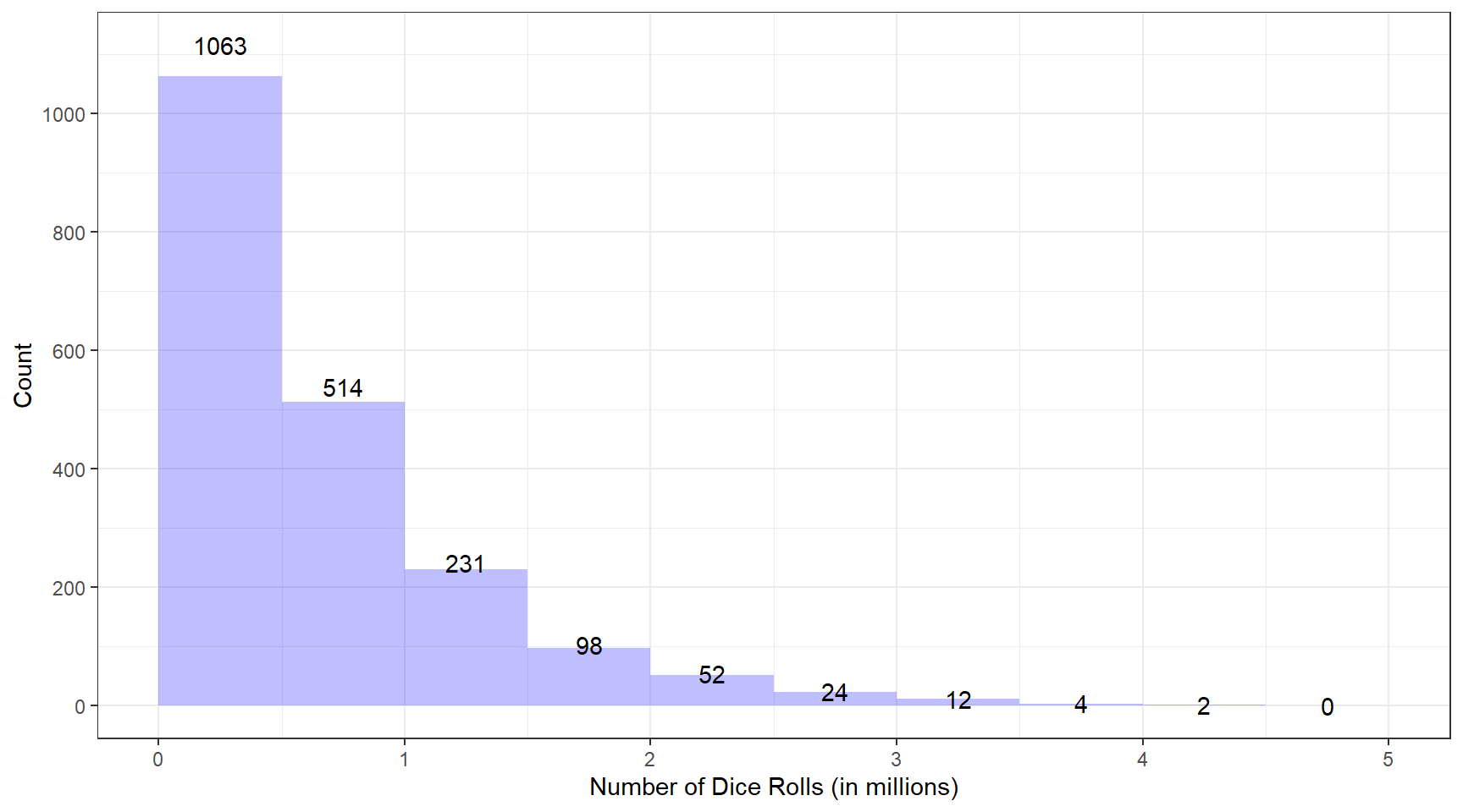 Noticeably, these data are right-skewed (skewness estimate of 1.7978162). Our standard five-number summary in summarizing these data is:
summary(data)## Min. 1st Qu. Median Mean 3rd Qu. Max.
## 44 183009 444204 642058 891602 4145846Thus 25% of the time (roughly 500 of the 2000 trials), we have up to 183,000 or so rolls; and about 50% of the time, we have up to around 445,000 rolls. This is an astonishing amount of variability; one would hope that these estimates would stabilize eventually. On average, we have an estimate of around 642,000 rolls; however, one must keep the variability in these data in mind when attempting to interpret this average.
Obviously, if I have more time available, I will increase the number of trials for this simulation.
Extending to 100,000 trials
Thank you, again, to David, who has run 100,000 trials of the above code. Below we show a histogram and five-number summary of these data.
vec <- eval(parse("dnd.txt"))
ggplot(data.frame(x = vec), aes(x = x)) +
  geom_histogram(breaks = seq(0, 5e6, 500000),
                 fill = "blue",
                 alpha = 0.25) +
  stat_bin(aes(y = ..count.., label = ..count..),
           geom="text",
           breaks = seq(0, 5e6, 500000),
           position = position_stack(vjust = 1.05)) +
  scale_x_continuous(labels = function(x) { x/1e6 }) +
  scale_y_continuous(breaks = seq(0, 60000, 10000)) +
  theme_bw() +
  ylab("Count") +
  xlab("Number of Dice Rolls (in millions)")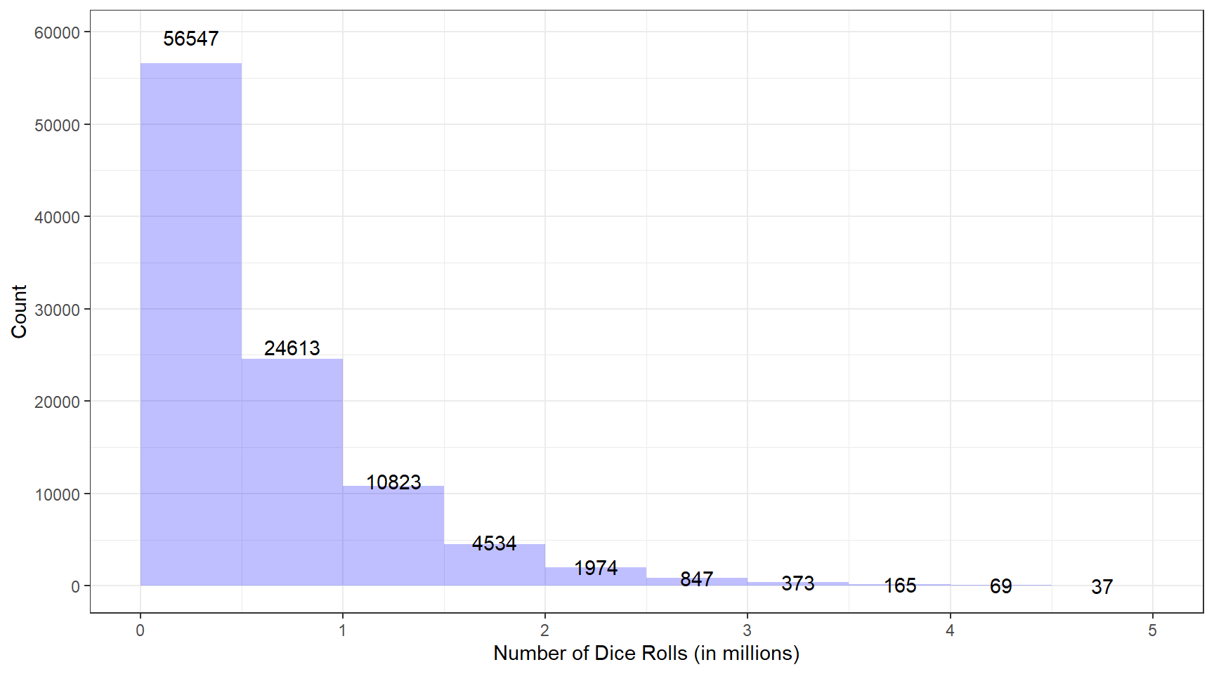
summary(vec)## Min. 1st Qu. Median Mean 3rd Qu. Max.
## 9 171488 415741 597603 831499 7876177Previously, 25% of the time, we had up to about 180,000 rolls; this time, it’s up to about 172,000. While these estimates are still quite different, in the grand scheme of things, these are relatively close.
The median last time was 445,000 rolls; now it’s about 415,700 rolls. Additionally, the mean was around 642,000 rolls last time; now it is around 600,000 rolls.
75% of the time last time, we had around 890,000 rolls; now, it is more like 830,000.
Conclusion: What do the data suggest?
Regardless of how far these two estimates are, one thing is clear: about 50% of the time, it will take roughly 420,000 rolls to “win” the game; and about 75% of the time, it will take 850,000 or so rolls to “win” the game. That is a lot of rolling!
Some Comments on Theory
One can observe this is a Markov chain, where the states can all be given by rolling the given dice as well as the finishing state, and the only possible transitions are d4 to d4, d4 to any one of the other die, and d20 to an ending state of finishing the game. I am not as familiar with the theory of stochastic processes as I’d like, but I would imagine additional insight can be provided there.
I would speculate we should be able to compute our five-number summaries exactly using some of the theory from Markov chains.
Yeng Miller-Chang
I am a student in the Georgia Tech OMSCS. Views and opinions expressed are solely my own.