An Exact Solution to "The Dice Game" using R, Python, and Markov Chains

Mathematical Theory

The Dice Game can be represented as a seven-state discrete-time Markov chain whose transition matrix is given by \[\mathbf{P} = \begin{array}{cc} \begin{array}{c} \end{array} & \begin{array}{ccccccc} \text{d}4 \hspace{1cm} & \text{d}6\hspace{0.25cm} & \text{d}8 \hspace{0.25cm}& \text{d}10\hspace{0.25cm} & \text{d}12 \hspace{0.25cm}& \text{d}20\hspace{0.25cm} & \text{win} \end{array} \\ \begin{array}{c} \text{d}4 \\ \text{d}6 \\ \text{d}8 \\ \text{d}10 \\ \text{d}12 \\ \text{d}20 \\ \text{win} \end{array} & \left[\begin{array}{ccccccc} 3/4 & 1/4 \\ 5/6 & & 1/6 \\ 7/8 & & & 1/8 \\ 9/10 & & & & 1/10 \\ 11/12 & & & & & 1/12 \\ 19/20 & & & & & & 1/20 \\ & & & & & & 1 \end{array}\right] \end{array}\text{.}\] All blank cells above are assumed to be \(0\).

To understand how to interpret the above, we represent transitions between the dice rolls by starting from the left and making our way up. For example, assuming you’re currently rolling the d4 (left side of the matrix), the probability that you will be rolling a d4 subsequently (top of the matrix) is \(3/4\) (i.e., you will roll the d4 again if you don’t obtain a 4). Similarly, assuming you’re currently rolling the d4 (left side of the matrix), the probability you will be rolling a d6 subsequently (top of the matrix) is \(1/4\) (i.e., you will roll the d6 if you roll a 4 on the d4).

A fact of Markov chains is that if \(\mathbf{P}\) is a transition matrix for one transition (as given above), then \(\mathbf{P}^n\) is the transition matrix for \(n\) transitions, with \(n \geq 1\) an integer.

The desired probability we seek can be described using linear algebra; namely, consider the fact that the probability we seek, from a \(1\)-step transition, is given by \[\underbrace{\begin{bmatrix} 1 & 0 & 0 & 0 & 0 & 0 & 0 \end{bmatrix}\mathbf{P}}_{\text{the d4 row}}\begin{bmatrix} 0 \\ 0 \\ 0 \\ 0 \\ 0 \\ 0 \\ 1 \end{bmatrix} = \mathbf{u}^{T}\mathbf{P}\mathbf{v} = \mathbf{P}_{\text{d4}, \text{win}}\text{.}\] The corresponding element of \(\mathbf{P}^n\) is thus \(\mathbf{u}^{T}\mathbf{P}^n\mathbf{v} = \mathbf{P}^n_{\text{d4}, \text{win}}\). However, note that this probability is cumulative in that it describes the probability that a transition is made from d4 to the win state within \(n\) transitions, not strictly at \(n\) transitions.

The probability of d4 to winning in one transition (though obviously \(0\)) is \(\mathbf{P}_{\text{d4, win}}\). In two transitions, \(\mathbf{P}^2_{\text{d4, win}}\) would contain the probability of a d4 to a win within two transitions, not strictly at two transitions. Thus, the probability of a d4 to a win in exactly two transitions is \(\mathbf{P}^2_{\text{d4, win}} - \mathbf{P}_{\text{d4, win}}\).

Similarly, the probability of a d4 to a win in exactly three transitions \(\mathbf{P}^3_{\text{d4, win}} - \mathbf{P}^2_{\text{d4, win}}\) since we must consider the differences between the probabilities within three transitions and the probabilities within two transitions to yield the probability of exactly three transitions.

Thus, the probability of a transition being made from d4 to the win state in exactly \(n\) transitions is \[p(n) = \mathbf{P}^n_{\text{d4, win}} - \mathbf{P}^{n-1}_{\text{d4, win}}\] for each \(n \geq 2\), and \(p(1) = \mathbf{P}_{\text{d4, win}}\). Obviously, \(p(1)\) through \(p(5)\) will all be \(0\) since a minimum of \(6\) transitions is necessary to win the game.

It is also worth noting that \(\mathbf{P}^n_{\text{d4, win}} = P(n)\) is the cumulative distribution function of the number of rolls it takes to win the game. Thus, we may compute \(P(n)\) and then compute pairwise differences to compute \(p(n) = P(n) - P(n-1)\).

Programming

The logical question to consider next is how large \(n\) needs to be so that the sum of the probabilities (considering floating-point error in R) is close enough to \(1\). Equivalently, what large value \(N\) do we need so that \(P(N) \approx 1\)?

In each time I ran the above computation for \(P(n)\), the probabilities were close to \(1\) for R at roughly \(N = 22,806,186\) rolls. Thus, I computed \(P(n)\) from \(n = 1\) to 23 million using R, and took pairwise differences to compute \(p(n)\) from \(n = 1\) to 23 million. I then saved this information into a table so that I would not have to worry about running this code again.

library(expm)

A <- matrix(
  c(  3/4, 1/4,   0,    0,     0,     0,    0,
      5/6,   0, 1/6,    0,     0,     0,    0,
      7/8,   0,   0,  1/8,     0,     0,    0,
     9/10,   0,   0,    0,  1/10,     0,    0,
    11/12,   0,   0,    0,     0,  1/12,    0,
    19/20,   0,   0,    0,     0,     0, 1/20,
        0,   0,   0,    0,     0,     0,    1),
  nrow = 7,
  ncol = 7,
  byrow = TRUE
)

mat_power <- function(A, n) {
  A %^% n
}

# around 23 million is fine
# exact: 22,806,186
end_idx <- 23000000
init_state <- 1
final_state <- 7

# Compute the CDF and the PMF
rolls_cdf <- sapply(X = 1:end_idx, 
                    FUN = function(x) { mat_power(A, x)[init_state, final_state] })
rolls_pmf <- c(0, diff(rolls_cdf))
rm(init_state, final_state)
rm(mat_power)
rm(A)

# Throw into a single table
df <- data.frame(
  x = 1:end_idx,
  cdf = rolls_cdf,
  pmf = rolls_pmf
)
rm(rolls_cdf, rolls_pmf, end_idx)
write.table(df, "20220211_exact_sim.txt", row.names = FALSE)

Of course, we will run into floating point errors, but it is worth performing some initial visualizations to make sure that what we output looks reasonable. R’s plotting functions are extremely slow given the number of points we are trying to plot, so we instead use the reticulate package to load Python into R, using matplotlib to do our plotting.

We combine R and Python code via the reticulate package to generate an image of the CDF \(P(n)\) using matplotlib.

library(data.table)
library(reticulate)
library(png)

df <- fread("20220211_exact_sim.txt")
Sys.setenv(RETICULATE_MINICONDA_PATH = "C:/MincondaPython39")
# py_install("matplotlib")
# py_install("pandas")

import pandas as pd
df = pd.DataFrame.from_dict(r.df)

import matplotlib as mpl
import matplotlib.pyplot as plt
mpl.use('Agg')
plt.rcParams['agg.path.chunksize'] = 0

plt.figure()
df.plot(x = "x", y = "cdf", legend = None)
plt.xlabel("Number of Rolls (in tens of millions)")
plt.ylabel("Cumulative Distribution Function")
plt.show()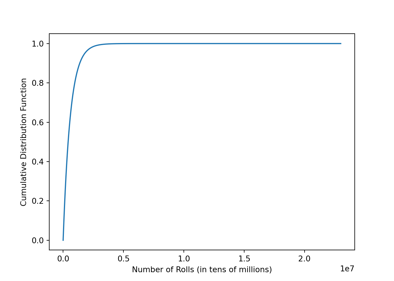

plt.close(plt.gcf())

Visually, this appears to meet all of the properties of a valid CDF: it is non-decreasing, has left-infinite limit of \(0\), and a right-infinite limit of \(1\).

The CDF looks reasonable, so then we plot the PMF.

plt.figure()
df.plot(x = "x", y = "pmf", legend = None)
plt.xlabel("Number of Rolls (in tens of millions)")
plt.ylabel("Probability Mass Function (divided by 10^(-5))")
plt.show()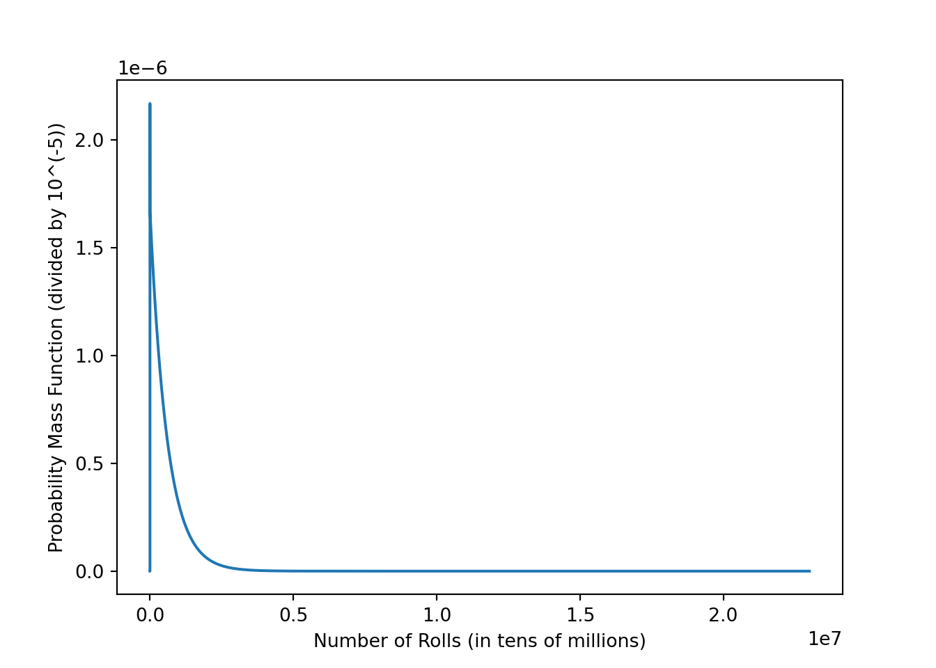

plt.close(plt.gcf())

This PMF appears to roughly align with what we observed previously via Monte Carlo simulation.

Statistical Computations

We can use basic probability to compute some quantities we would be interested in.

Question 1: How many rolls would you need to win the game 25% of the time?

min(which(df$cdf >= 0.25))

## [1] 171997

Question 2: Extend question 1, but now for 50%, 75%, 95%, and 99% of the time?

# 50% 
min(which(df$cdf >= 0.5))

## [1] 414407

# 75%
min(which(df$cdf >= 0.75))

## [1] 828808

# 95%
min(which(df$cdf >= 0.95))

## [1] 1791018

# 99%
min(which(df$cdf >= 0.99))

## [1] 2753228

Question 3: What is the average number of rolls we would expect to roll to win?

Recalling from probability that the expected value is given by \[\mathbb{E}[X] = \sum_n n \cdot p(n)\] we thus have

sum(df$x * df$pmf)

## [1] 597860

Conclusion

If you want to win The Dice Game:

• 25% of the time, you should expect to roll your dice 171,997 times.
• 50% of the time: 414,407 times.
• 75% of the time: 828,808 times.
• 95% of the time: 1,791,018 times.
• 99% of the time: 2,753,228 times.

The average (mean) number of times you should expect to roll is 597,860 times.